10 Sep 2015

A Stochasitic Method for Solving L1 Regularized Optimization Problem

Introduction

In machine learning, regularization are an usual method for model adjustment, in particular to prevent overfitting by penalizing models with extreme parameter values. Regularzation is critical to training machine learning models so that different regularization terms lead to total different model parameters. The most common used variants are L1 and L2 regularization terms, which should be appended to objective optimization functions. This article focus on solving optimization problems with L1 regularization term.

As you know, L1 regularization refers to the L1-Norm of parameter values, which could generate sparsity. To construe sparsity, suppose each sample in a given training set contains tens of thousands dimensions(some dimensions can be a combination of others) to model an intricate interaction relationship in real world. After finishing training the model, you will get a high-dimensional weight vector corresponding to relative data dimension. You tell yourself this weight vector is good(not overfitting) and will perform well in future prediction work. But actually you know little about the weight values and may feel it like a black box. Unlike other regularizations, L1 regularization strategy will do model selection automaticly and will always return a sparse weight vector. This kind of sparsity make sense, because some input dimensions have no influence with the output value. If original dimensions of input data have some real meanings, it leads to interpretability and it is a rather attractive property of L1 regularization.

The Problem

L1 regularized optimization problem is defined below: $$ \mathsf {\min}_{w \in R^{d}} \ f(w), \ f(w)=\frac{1}{m} \sum_{i=1}^{m} L(\langle w, x_{i} \rangle, y_{i}) + \lambda \Arrowvert w \Arrowvert_{1} \ \ (1) $$ where \( \lambda>0 \) is regularization parameter. The generic problem includes as special cases the Lasso(Tibshirani, 1996), in which \( L(a, y) = \frac{1}{2} (a-y)^{2}\), and logistic regression, in which \( L(a, y) = log(1 + exp(-ya)) \). For simplicity, let’s assume that \( L \) is convex w.r.t. its first argument so that Eq(1) is a convex optimization problem, and therefore can be solved using standard optimization techniques, such as interior point methods and so on. However, standard methods prove to scale poorly with the size of the problem(i.e. \( m \) and \( d \), so in stead, we’d better choose a stochastic method.

Another challenge in solving L1 regularized optimization problem is that traditional defined gradients of objective functions do not exist, that’s the reason L2 regularization is much more widely used. As far as we know, there are two ideas for solving L1 regularized optimization problems. Firstly, some algorithms transform original problem into another form, and in new space the problem becomes derivable. The other class of algorithms define a generalized form of function derivative(with special property) then solve the original problem directly. These tricks are being actively researched in the near decade since 2000 but in this article we will only discuss an algorithm following the former idea.

Transformation

Because derivative of loss functions in Eq(1) is hard to calculate, we try to transform original problem. We will start by giving some intuitions. Firstly, there is a trick for representing a real number by the Lemma given below:

Lemma1. For an arbitrary real number w, there exists the only pair \( v_{p} \) and \( v_{n} \), satisfies \( v_{p} \geq 0, v_{n} \geq 0 \) and \( v_{p} \cdot v_{n} = 0, s.t. w = v_{p} - v_{n} \).

Proof. The existence of \( v_{p} \) and \( v_{n} \) is obvious. If w is positive, let \( v_{p} = w , v_{n} = 0 \), if w is negative, let \( v_{p} = 0, v_{n} = -w \), and satisfies \( v_{p} \cdot v_{n} = 0 \) such that \( w = v_{p} - v_{n} \). To prove the uniqueness, without loss of generality, suppose w is positive. Because \( v_{p} \cdot v_{n} = 0 \), if \( v_{n} = 0 \), then \( v_{p} = w \) and it is good. If \( v_{p} = 0 \), we will get \( v_{n} = -w < 0 \) which violates the condition \( v_{n} \geq 0 \).

An obvious corollary of lemma1 is: \( |w| = v_{p} + v_{n} \), so by using this trick, we successfully remove the absolute symbol for \( w \). And therefore, for a given real number \( w_0 \), $$ \mathsf f(w_{0}) = \frac{1}{m} \sum_{i=1}^{m} L(\langle w_{0}, x_{i} \rangle, y_{i}) + \lambda \Arrowvert w_{0} \Arrowvert_{1} $$ $$ \mathsf = \frac{1}{m} \sum_{i=1}^{m} L(\langle [v_{0p}, -v_{0n}], x_{i} \rangle, y_{i}) + \lambda \Arrowvert [v_{0p}, -v_{0n}] \Arrowvert_{1} $$ $$ \mathsf = \frac{1}{m} \sum_{i=1}^{m} L(\langle v_{0p}, x_{i} \rangle + \langle v_{0n},, -x_{i} \rangle, y_{i}) + \lambda \Arrowvert [v_{0p}, -v_{0n}] \Arrowvert_{1} $$ $$ \mathsf = \frac{1}{m} \sum_{i=1}^{m} L(\langle v_{0}, [x_{i}, -x_{i}] \rangle, y_{i}) + \lambda \sum_{i=1}^dv_{0_{i}} $$ $$ \mathsf v_{0_{i}} \geq 0, v_{0_{k}} \cdot v_{0_{k+d}} = 0 \ with \ i \in [1, 2d] \ and \ k \in [1,d] $$ After that, we try to define a transformation problem, which is a constraint optimization problem as: $$ {\min}_{v \in R^{2d}} \ g(v), \ g(v) = \frac{1}{m} \sum_{i=1}^{m} L(\langle v, [x_{i}, -x_{i}] \rangle, y_{i}) + \lambda \sum_{i=1}^dv_{i} \ \ (2) $$ $$ \mathsf v_{i} \geq 0, v_{k} \cdot v_{k+d} = 0 \ with \ i \in [1, 2d] \ and \ k \in [1,d] $$ To prove that solution \( v^{\star} \) of Eq(2) is equivalent to solution \( w^{\star} \) of Eq(1), let’s suppose \( w^{\star} \) is the solution of Eq(1) and the minimum loss value is \( f(w^{\star}) = C \), then we have \( v^{\star} \) satisfies Lemma1. If \( v^{\star} \) is not the solution of Eq(2), there must exists another \( v^{\star’} \) such that \( g(v^{\star’}) = C^{‘} < C \). Therefore, we can find \( w^{\star’} \) such that \( f(w^{\star’}) = C^{‘} < C \), which generates conflicts and vice versa.

Now we have a transformed constraint optimization problem which is equivalent to the original optimization problem. There are two restricted conditions of Eq(2) so far: \( v_{i} \geq 0 \) and \( v_{k} \cdot v_{k+d} = 0 \ with \ i \in [1, 2d] \ and \ k \in [1,d] \). In fact, the latter condition is implicitly included so can be removed. To explain that, let’s define a problem without the restriction of this condition. Suppose the solution of this problem is \( v^{\star\star} \in 2d \) which is not equal to \( v^{\star} \) which is the solution for Eq(2). Reorganize the order of its 2d dimensions with \( [v^{\star\star}_{i}, v^{\star\star}_{i+d}] \), since \( v^{\star\star}_{i} \cdot v^{\star\star}_{i+d} \neq 0 \), we can construct a new vector \( u^{\star} \) with \( u^{\star}_{i} = v^{\star}_{i} - v^{\star}_{i+d}, u^{\star}_{i+d} = 0(u^{\star}_{i} \geq u^{\star}_{i+d}) \ or \ u^{\star}_{i} = 0, u^{\star}_{i+d} = v^{\star}_{i} - v^{\star}_{i+d} (u^{\star}_{i} \leq u^{\star}_{i+d}) \). It is clear that \( u^{\star} \) is a better solution of the problem which generates conflicts. Till now, we can define the ultima transformed problem which only contains one restricted condition as: $$ {\min}_{v \in R^{2d}} \ g(v), \ g(v) = \frac{1}{m} \sum_{i=1}^{m} L(\langle v, [x_{i}, -x_{i}] \rangle, y_{i}) + \lambda \sum_{i=1}^dv_{i} \ \ (3) $$ $$ \mathsf v_{i} \geq 0\ with \ i \in [1, 2d] $$

Stochastic Coordinate Descent

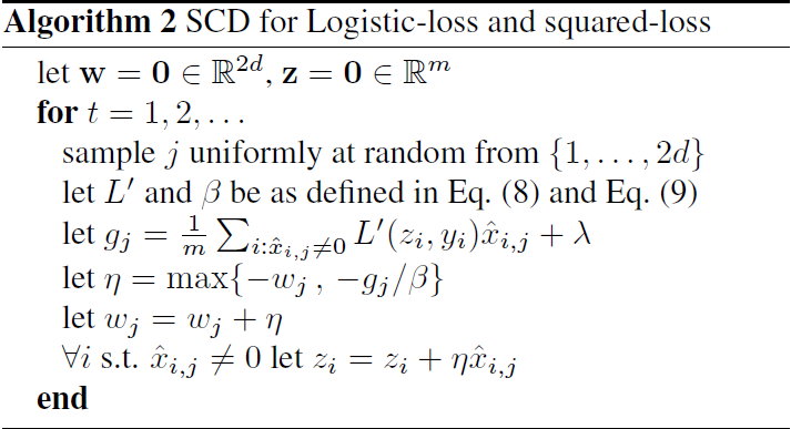
In last section, we find a transformed constraint optimization problem, and if we solve Eq(3), we can easily construct the solution of Eq(1). In this section, we will present an simple algorithm called stochastic coordinate descent to solve Eq(3).

The algorithm initializeds \( w \) to be 0, at each iteration, it picks a coordinate \( j \) uniformly at random from \( [1, 2d] \). Then the derivative of loss functions w.r.t. the \( j \)th element of \( w \), \( \delta_{k} = \bigtriangledown{g(w)_{k}} \) is calculated. Next, a step size is determined based on the value of \( \delta_{k} \) and a parameter of the loss function denoted \( \beta \). This parameter is an upper bound on the second derivative of the loss. The step size is trimmed so as to ensure that after performing the update, the constraint \( w_{k} \geq 0 \) will not be violated. Finally, we update \( w_{k} \) according to the calculated step size. For square-loss function \(L\), \( \beta \) is set with 1 and for logistic-loss function \(L\), \(\beta\) is usally set with \(\frac{1}{4}\).

The stochastic coordinate descent algorithm showed above is similar to the stochastic gradient descent algorithm. In stead of choosing a training sample, SCD randomly chooses a dimension and updates that dimension parameter using derivative information. You can read the reference of Shalev-Shwartz S, Tewari A. Stochastic methods for l 1-regularized loss minimization[J]. The Journal of Machine Learning Research, 2011, 12: 1865-1892 to see more details such as convergent speed and so on.

Implementation

Implement the SCD algorithm for solving Eq(3) is very straightforword. The note you need to pay attention to is that you may firstly transform d-dimensional input data to 2d-dimension, but actually you don’t need to store the 2d-dimensional vector at all. After training, you also need to convert the 2d-dimensional vector into d-dimensional parameter vector of the original problem. We wrote a sequential SCD version of lasso and L1-regularized logistic regression inside paracel framework, you can run the code following the documents here.

For a small lasso test, we created a small traning set containing 10000 samples with 100 dimensions, after training about 2000 iterations, we got the parameter vector as \([0,…,0,14.405463,0,…,0,94.507575,0,…,0,37.381599,\) \(0,…,0,68.744748,0,…,0,20.467441,0,…,0,69.616527,\) \(0,…,0,58.277555,0,0,42.087466,30.840373,0,…,0,\) \(32.190664,0,…,0.000003,0,…,0]\), you can see there are lots of zeros in the vector. You can then use paracel framework to extend the sequential version to a distributed version to handle big data. More technical details for distributed SCD algorithm can be found in Bradley J K, Kyrola A, Bickson D, et al. Parallel coordinate descent for l1-regularized loss minimization[J]. arXiv:1105.5379, 2011.

Conclusion

In this article, we introduce the L1 regularized optimization problem and discuss two basic ideas for solving that problems. Following the first kind, we transform original problem to a constraint optimization problem and use an simple stochasitic algorithm called SCD to train the model. We also showed you two sequential implementations of lasso and l1 regularized logistic regression solvers. Hope you can enjoy this blog.

Hong Wu at 11:37